How does production line speed affect in-line measurement accuracy?

How does production line speed affect in-line measurement accuracy?

Increasing production line speed reduces the time available for in-line measurement, but faster throughput does not automatically mean lower accuracy. The outcome depends on sensor response time, sampling rate, exposure or integration time, synchronization, and product stability. The practical question is whether the complete measurement system can resolve critical features and maintain acceptable uncertainty at the intended operating speed.

A gauge that performs well on a stationary reference may struggle on a vibrating strip. Conversely, a properly triggered optical system can maintain reliable dimensional results as throughput rises—until exposure, lighting, processing, or mechanical limits become restrictive. Evaluating that boundary requires more than comparing the accuracy figures in supplier datasheets.

Speed changes the measurement window, not just the reading rate

For a moving product, the available observation time depends on both velocity and the length over which a valid measurement can be taken:

Available measurement time = usable measurement length ÷ line speed

As a purely illustrative calculation, a 20 mm usable measurement zone at 2 m/s provides 10 ms. That interval must accommodate whatever the application requires: settling, illumination, signal integration, or collection of enough valid samples. It is not necessarily the total time available for downstream processing, which may continue after the product leaves the sensor.

The meaning of “usable” matters. On a checkweigher, it may be the period during which the item is fully supported by the weighing conveyor without touching adjacent belts. On a vision station, it may be the field region where distortion and lighting remain acceptable. Using the entire physical sensor zone in the calculation can overstate the available measurement window.

Where speed-related errors actually enter

Sensor response and filtering can hide short events

A fast communications interface does not prove that the sensing element responds equally quickly. A transmitter can publish frequent values while its sensing element or digital filter responds much more slowly. Consecutive readings may therefore contain little new information.

For an approximately first-order sensor, the time constant describes how quickly its output approaches a changed input; after one time constant, the response reaches about 63% of a step change. Real instruments may have more complicated dynamics. If a moving feature passes before the system responds sufficiently, its measured peak can be attenuated or its apparent position shifted.

Filtering creates a similar trade-off. More averaging may improve repeatability on a uniform product but suppress a narrow thickness excursion. A smoother trace is not necessarily a more faithful measurement.

Sampling density determines what can be resolved

For uniformly timed samples at constant speed, the nominal distance between measurements is:

Spatial sample spacing = line speed ÷ sampling frequency

In an illustrative setup, 2 m/s motion and a 1 kHz acquisition rate produce 2 mm spacing. That may suit broad profile changes but cannot reliably characterize a 1 mm defect. Even when a feature occasionally coincides with a sample, detection may depend on its position relative to the sampling sequence.

Do not turn the Nyquist criterion into a blanket “two samples per defect” rule. It applies to band-limited signals under defined conditions. Reliable edge location, peak measurement, and isolated-defect detection generally require application-specific sampling density, adequate sensor bandwidth, and consideration of the sensor’s spatial footprint.

Exposure trades motion blur against signal quality

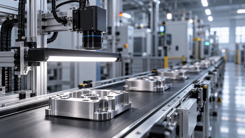
For optical inspection, approximate object-space motion during exposure is line speed multiplied by exposure time. At 2 m/s, an illustrative 100 microsecond exposure corresponds to 0.2 mm of travel. Whether that is acceptable depends on magnification, feature geometry, contrast, and the measurement algorithm.

Shortening exposure reduces motion blur but also reduces collected light unless illumination changes. Noise may then destabilize edge detection. Strobing, suitable optics, and a global-shutter camera can help, but each has limits. A higher frame rate alone does not solve blur, and a rolling shutter can introduce geometric distortion during motion.

Synchronization errors can look like sensor inaccuracy

A correct measurement attached to the wrong location or product is still a failed inspection. Trigger timing, encoder scaling, timestamps, PLC scan behavior, and network delays all affect whether a reading is associated with the intended feature.

Under constant-speed conditions, timing uncertainty translates into position uncertainty approximately as position uncertainty = speed × timing uncertainty. Fixed latency and variable latency deserve different treatment: a predictable delay can often be compensated, while timing jitter creates variable position error. During acceleration, compensation must account for changing velocity rather than assuming a constant travel time.

Encoder-triggered acquisition is often preferable when spatial spacing matters and line speed varies. However, an encoder on a drive shaft does not necessarily track actual product motion if belt slip, stretch, or product sliding occurs. Check the mechanical relationship before treating encoder counts as ground truth.

The reject station adds another timing problem. Detection may work perfectly while the actuator rejects the next item. Validation should follow the result through acquisition, decision, product tracking, and physical rejection—not stop at the sensor output.

Sometimes the product changes faster than the instrument does

Higher speed can change vibration, web flutter, belt tension, product orientation, or liquid presentation. A laser displacement sensor may accurately detect surface movement while the application incorrectly interprets that movement as thickness variation. Opposed sensors or a controlled reference geometry may be necessary to separate thickness from vertical displacement.

On a filling line, sloshing, foam, and bubbles can alter level or optical signals. In continuous processing, a throughput increase may change temperature, pressure, flow profile, or mixing conditions. These are not all instrument errors: some represent genuine changes in the measurand or in how representative the sensing location is.

That distinction affects the remedy. Buying a faster sensor will not remove mechanical instability or correct an unrepresentative sampling point. Sometimes the better investment is a guide, isolation mount, improved product spacing, or a different measurement location.

Read specifications as a connected measurement chain

When comparing in-line measurement systems, ask which specifications apply simultaneously. Maximum sampling rate, best repeatability, and highest resolution may come from different operating modes. At Global Instrument Hub (GIH), this distinction is central to useful instrumentation intelligence: component specifications need to be interpreted against the complete application, not ranked in isolation.

• Response specification: Is it sensing-element response, filtered output settling time, or merely the communications update interval?
• Acquisition conditions: What exposure, integration time, averaging, measurement range, and target surface produced the stated performance?
• Sustained processing: Can the system inspect continuously with the required algorithms, data logging, and interfaces enabled?
• Invalid-result handling: Are saturation, missed triggers, low signal, and buffer overflow explicitly flagged, or can stale values appear valid?
• Latency behavior: Are both typical delay and its variation specified under realistic operating load?

An invalid reading should not silently become a passing result. This is especially important when higher speed pushes illumination, computation, or communications close to capacity.

Validate the operating envelope, not one nominal speed

Begin with the measurement task: the quantity being measured, tolerance, smallest relevant feature, and consequences of a false acceptance or false rejection. “Detect defects at maximum speed” is not a sufficient acceptance criterion.

Use representative products with independently established reference values and documented reference uncertainty. Include difficult surfaces, relevant size extremes, and samples near specification limits. Where practical, measure the same items repeatedly at low, nominal, and maximum speed so that product variation does not obscure speed-related effects.

Then test acceleration, deceleration, minimum spacing, normal vibration, and sustained production. Record measurement bias and repeatability separately from missed detections, invalid readings, and tracking errors. A system may show little average bias while its occasional failures make it unsuitable for automatic release.

Build the uncertainty assessment around actual operating conditions. JCGM 100, the Guide to the Expression of Uncertainty in Measurement, provides a general framework; it does not prescribe a universal line-speed limit. Contributions may include reference uncertainty, calibration, dynamic response, alignment, temperature, and timing. Avoid double-counting effects already captured by representative repeatability testing.

ISO/IEC 17025 addresses laboratory competence and supports confidence in relevant calibration or testing work; an accredited calibration alone does not validate an installed production-line system. Applicable instrument-specific, contractual, or legal-metrology requirements must also be checked. Where conformity decisions are made near tolerance limits, agree on the decision rule and any guard band before acceptance testing.

Set the speed limit from demonstrated performance

There is no universal percentage by which accuracy deteriorates as line speed rises. The limiting mechanism may be blur on one line, settling time on another, and product tracking on a third. Reducing speed is justified when it restores required performance, but it should follow diagnosis rather than replace it.

The most useful acceptance output is a validated operating envelope: permitted speed, product spacing, material conditions, acquisition settings, uncertainty, and failure-handling behavior. Preserve those settings under change control. If production later changes lighting, filtering, conveyor geometry, or product format, reassess the affected limits rather than assuming the original speed approval still holds.