How does temperature affect high-accuracy sensor performance?


A high accuracy sensor can meet its laboratory specifications yet produce unacceptable errors when its temperature changes. Temperature can shift the zero point, alter sensitivity, increase noise, and create mechanical stresses that persist after the temperature returns to its starting value. Accuracy at a reference temperature is therefore not the same as accuracy across an operating temperature range.
The decisive question is whether the complete measurement system stays within its allowable uncertainty under the temperatures, gradients, and rates of change it will actually experience. Answering that requires more than checking an operating-temperature limit: it requires understanding thermal error specifications, compensation boundaries, and installation conditions.
Temperature changes both the offset and the measurement scale
A useful simplified model for a sensor calibrated at reference temperature T₀ is:
Indicated value ≈ [1 + g(T)] × actual input + b(T)
Here, b(T) is the temperature-dependent offset expressed in measurement units, and g(T) is the fractional sensitivity error. Both represent changes relative to calibration at T₀. This model does not capture every effect, but it separates two errors with different consequences.
Zero or offset drift changes the output even when the measured input remains zero. In a pressure sensor, the indicated pressure may move with temperature despite no change in applied differential pressure. An offset specified as a percentage of full scale can dominate the error when measuring near the bottom of the range.
Sensitivity or span drift changes the relationship between input and output. A sensor may remain correct at zero but increasingly misread as the input rises. A zero adjustment cannot remove this error; measurements at multiple input levels are needed to identify it.
Near the reference temperature, manufacturers may describe these effects using temperature coefficients. Over a wider interval, their behavior can be nonlinear. A single coefficient is useful only within the range and conditions for which it is specified.
The physical source of thermal error depends on the sensor
Temperature affects the sensing element, its packaging, and the electronics that convert its response into a usable signal. Identifying the dominant mechanism helps determine whether compensation, mechanical changes, or thermal control will be effective.
Noise must be distinguished from drift. Averaging can reduce some random fluctuations, but it does not remove a temperature-dependent bias. Stronger filtering may make a drifting reading look more stable while also concealing a real process change.
Temperature can also change the quantity being measured. A sealed gas volume changes pressure as its temperature changes; a metal target changes dimensions through thermal expansion. These are physical changes in the measurand, not necessarily sensor errors. The measurement requirement must specify whether the desired result is the value at operating conditions or a value corrected to a reference temperature.
Uniform temperature and thermal gradients are different problems
A chamber specification generally describes performance under defined thermal conditions. An installation may expose the sensing diaphragm to hot process fluid while the electronics remain near room temperature. A load cell may be warmed on one side by machinery and cooled on the other by airflow.
Such gradients create differential expansion, package stress, and internal temperatures that are not represented by a single ambient reading. Two installations at the same nominal ambient temperature can therefore produce different errors.
Transient conditions create another limitation. The sensing element, housing, compensation sensor, and electronics have different thermal time constants. During rapid heating or cooling, the temperature used for correction may lag behind the component producing the error. A steady-state compensation map cannot necessarily correct that mismatch.
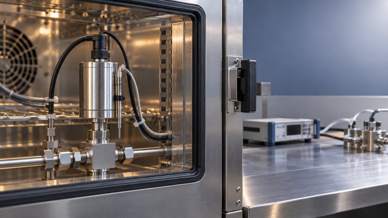
Thermal hysteresis adds a history-dependent effect: at the same input and temperature, the output can differ depending on whether the assembly was heated or cooled. Packaging stress, adhesive behavior, and mechanical interfaces can contribute. A non-recovering shift after cycling should also be distinguished from reversible thermal drift, because returning to the reference temperature may not restore the original calibration.
Read temperature specifications as separate performance claims
Temperature-related entries on a datasheet answer different questions. Treating them as interchangeable can lead to a substantial understatement of measurement error.
- Operating temperature range: the interval in which operation is permitted under stated conditions. It does not, by itself, guarantee reference-temperature accuracy.
- Compensated temperature range: the interval over which specified compensation performance applies. Residual error remains.
- Reference-temperature accuracy: an error specification at a stated temperature or narrow temperature interval. Its included components must be checked.
- Temperature coefficient of zero: offset change with temperature, often expressed relative to full scale rather than the current reading.
- Temperature coefficient of sensitivity: gain change with temperature, whose contribution depends on the applied input.
- Total error band: an envelope combining specified errors across defined conditions. Its definition must be read rather than assumed.
A total error band may include nonlinearity, hysteresis, repeatability, and thermal zero and span effects, but inclusion varies by manufacturer. Long-term drift, installation stress, dynamic thermal effects, or external electronics may remain outside it. Adding separate thermal coefficients to an envelope that already includes them can double-count errors; ignoring excluded effects can understate them.
Units matter just as much as labels. Percent of full scale, percent of reading, parts per million per kelvin, and measurement units per degree are not directly interchangeable. A temperature difference of one kelvin equals one degree Celsius, but the percentage denominator still determines the practical error.
A small coefficient can consume the entire error allowance
Consider an illustrative 0–100 bar sensor with a reference-temperature error limit of ±0.05% full scale. Suppose its zero temperature coefficient is bounded by ±0.01% full scale per °C over the relevant interval. At 30°C above the reference temperature, the zero contribution alone could reach:
100 bar × 0.0001/°C × 30°C = 0.30 bar
The reference-temperature error limit corresponds to only ±0.05 bar. At an actual pressure of 10 bar, the thermal zero contribution is equivalent to 3% of the reading, before other errors are considered.
This is a hypothetical calculation, not a product specification. It shows why a small full-scale percentage can be unacceptable at low input levels. It also assumes that the coefficient is a valid bound across the full temperature excursion; a typical coefficient or local slope cannot automatically support that calculation.
Compensation reduces error within a model—not under every condition
Digital compensation commonly uses calibration measurements at several temperatures and input levels to estimate correction coefficients. Analog approaches can balance selected temperature dependencies within the sensing bridge or conditioning circuit. Either method can reduce thermal error, but neither eliminates the need for a residual-error specification.
The important evidence is the performance after compensation: the covered temperature and input ranges, whether limits are guaranteed or typical, and whether characterization applies to individual devices or a representative population. Calibration-point density also matters where the thermal response is nonlinear.
Compensation becomes less reliable when operating conditions differ from its underlying model. Examples include gradients absent during calibration, rapid transients, changed mounting stress, or aging that alters the original relationship between temperature and output.
Power introduces another complication. Bridge excitation, internal electronics, and output loading can heat the device above ambient temperature. Changing the supply voltage, duty cycle, enclosure, or airflow can alter this temperature rise. Consequently, calibration and validation should use electrical operating conditions representative of service.
Build an uncertainty budget around the installed measurement chain
The measurement chain includes more than the sensor: excitation, wiring, connectors, signal conditioning, conversion, and mechanical installation can all contribute temperature-dependent errors. Low-level voltage measurements may be affected by thermoelectric voltages at dissimilar-metal junctions. Resistive measurements can be affected by lead resistance, depending on the connection method.
For each contribution, establish its magnitude, operating conditions, and relationship to other errors. Manufacturer maximum-error limits should not simply be combined by root-sum-square as though they were independent standard uncertainties.
A conservative error-limit assessment may add applicable bounds. A measurement uncertainty evaluation instead assigns justified distributions and sensitivity coefficients and accounts for correlations. The Guide to the Expression of Uncertainty in Measurement, JCGM 100, provides the general framework. Where a bounded input is reasonably modeled by a rectangular distribution, its half-width divided by √3 gives the associated standard uncertainty; that modeling assumption requires justification.
Known, significant biases should be corrected where practicable, with uncertainty assigned to the correction. Otherwise, the remaining bias must be addressed explicitly in the acceptance decision rather than hidden within an unexplained uncertainty total.
Validate thermal performance under conditions that reproduce the risk
A useful thermal evaluation measures several input levels at several temperatures, including the reference condition and the expected application extremes. Zero or low-input measurements expose offset changes; upper-range measurements reveal span changes. Intermediate points help identify nonlinear behavior.
Repeat measurements during both heating and cooling. Returning to the reference temperature after an excursion helps distinguish reversible drift from hysteresis or a residual shift. Where rapid temperature changes occur in service, include transient tests rather than relying solely on stabilized results.
Stabilization should be demonstrated by the device and its output, not inferred solely from the chamber reaching its setpoint. The reference measurement system must also remain sufficiently stable: heating a pressure source, fixture, or dimensional artifact can change the applied input and confound the result.
Record mounting torque, orientation, supply conditions, output loading, cable configuration, process-medium temperature, ambient temperature, and relevant internal temperature readings. These details define whether the result represents the intended installation.
IEC 60068-2-1, IEC 60068-2-2, and IEC 60068-2-14 address cold, dry heat, and change-of-temperature testing respectively. They provide environmental test methods, not a universal accuracy guarantee. A meaningful performance claim must identify test severity, measurement conditions, and acceptance criteria.
ISO/IEC 17025 addresses laboratory competence, impartiality, and consistent operation. Accreditation is relevant only within the laboratory’s accredited scope; it does not establish a sensor’s thermal accuracy by itself. Calibration evidence must cover the required quantities, ranges, conditions, and uncertainties.
The strongest basis for acceptance is a bounded residual error or defensible uncertainty result for the actual thermal envelope. If temperature effects consume the available allowance, the remedy may be a narrower sensor range, better thermal isolation, controlled warm-up, installation changes, or calibration across temperature—not simply a better headline accuracy figure.
Recommended for You
 How does temperature affect high-accuracy sensor performance?Explore how temperature affects high accuracy sensor performance. Learn to reduce thermal drift, evaluate compensation, and select the right sensor for reliable measurements.
 Can a C4H8O concentration analyzer distinguish between isomers?Can a C4H8O concentration analyzer distinguish isomers? Compare GC, FTIR and MS methods, uncover selectivity limits, and learn what to validate before choosing your instrument.
 How to identify a reliable supplier using on-time delivery recordsIdentify a Reliable Supplier by verifying on-time delivery records, original commitments, and complete shipments. Learn practical checks to reduce purchasing risk and protect your project schedule.
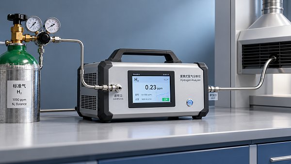
 How sensitive should a portable hydrogen analyzer be for lab use?Choose a portable hydrogen analyzer for laboratory use with the right quantification limit, accuracy, and range. Learn how to verify performance and avoid costly buying mistakes.
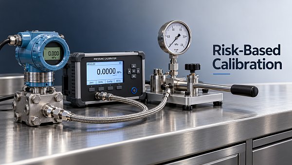
 How to set industrial calibration intervals based on equipment riskSet industrial calibration intervals based on equipment risk, drift, and as-found data. Learn when to shorten or extend schedules to improve reliability and avoid unnecessary costs.
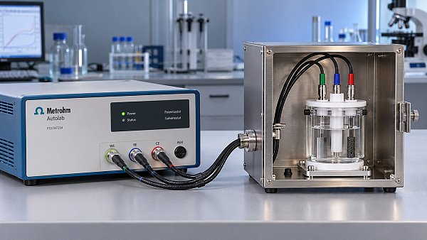
 How to choose electrochemical analyzers for low-current measurementsCompare electrochemical analyzers for precise low-current measurements. Learn how noise, leakage, bandwidth, and real-cell testing help you choose the right instrument.
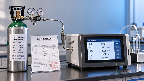
 What tolerance does a custom gas mixture need for calibration?Choose the right custom gas tolerance for calibration. Learn how blending tolerance, certified uncertainty, and stability affect accuracy—and avoid paying for precision you don’t need.
 How condensation affects stack detector readings in wet flue gasStack detector readings can drift when wet flue gas condenses. Learn how to identify moisture interference, prevent sample losses, and improve emissions monitoring reliability.
 How to prevent condensation in a CO2 analyzer sampling systemPrevent condensation in your CO2 analyzer sampling system. Learn how to control dew point, eliminate cold spots, and manage moisture for reliable readings and fewer costly disruptions.
 How to verify accuracy claims for industrial quality analyzersVerify accuracy claims for industrial quality analyzers with calibration checks, independent testing, and clear acceptance criteria. Learn how to reduce risk and buy with confidence.
 How to calculate cooling loads for an industrial analyzer shelterSize industrial analyzer shelter cooling with confidence. Learn to calculate equipment heat, solar gains, and ventilation loads, then select HVAC capacity for reliable analyzer performance.
 Hydrogen Analyzers for Energy Storage: Purity Monitoring vs. Leak DetectionChoosing a hydrogen analyzer for energy storage systems? Compare purity monitoring and leak detection to select the right sensors, improve safety, and protect fuel cell performance.
 NH3 Monitoring in Fertilizer Plants: Where Should Leak Analyzers Be Installed?NH3 analyzer for fertilizer production: discover where to place leak detectors around storage, compressors, and loading areas to reduce blind spots and improve early warning.
 Diesel Engine NOx Analyzers: Response Time and NO2 Conversion ExplainedChoosing a NOX analyzer for diesel engines? Learn how response time, NO2 conversion, and sampling design affect accuracy—and make a smarter, evidence-based purchase.
 SO2 Analyzers for Smelter Emissions: Sampling Hot, Dust-Laden Flue GasSelect an SO2 analyzer for smelting industry applications. Discover how to handle hot, dust-laden flue gas, prevent sample losses, and achieve reliable emissions monitoring.
 Unstable CH4 Readings in Biogas Monitoring? Check Moisture and Sample FlowCH4 analyzer for biogas monitoring giving unstable readings? Discover how moisture, sample flow, and pressure checks help pinpoint faults and restore reliable methane measurements.
 Buying a CO2 Analyzer for Brewery Gas Recovery: Costs Beyond the Purchase PriceBuying a CO2 analyzer for brewery applications? Compare sampling, installation, calibration, and downtime costs to uncover hidden expenses and make a smarter gas recovery investment.
 Where to Place CO Analyzers for Effective Parking Garage VentilationOptimize your CO analyzer for parking garage ventilation with practical placement tips. Learn how sensor height, airflow, and zone coverage support timely detection and effective fan control.
 NDIR vs. FTIR Gas Analyzers: Which Fits Your Environmental Research?Find the right infrared gas analyzer for environmental research. Compare NDIR vs. FTIR on sensitivity, gas coverage, sampling needs, and cost to choose confidently for your study.
 Oxygen Analyzers for Diving: Calibration Checks Before Nitrox BlendingUsing an oxygen analyzer for diving applications? Discover essential calibration, sensor, and sampling checks before nitrox blending to support reliable readings.
 How Paramagnetic Oxygen Analyzers Work and Why Sample Pressure MattersLearn how a paramagnetic oxygen analyzer works, why sample pressure affects accuracy, and what to check in compensation and calibration before choosing your system.
 How Much Does a Complete CEMS Integration Project Typically Cost?How much does a complete CEMS integration project typically cost? Explore budget ranges, hidden installation costs, and compliance needs to compare quotes and plan confidently.
 What Is the Typical Response Time for Industrial Air Monitors?What is the typical response time for industrial air monitors? Explore T90, sampling delays, and alarm settings to compare performance and choose the right monitor with confidence.
 Do Regulatory Monitoring Systems Need Third-Party Certification?Do regulatory monitoring systems need third-party certification? Learn when it is required, what certificates prove, and how to verify compliance before buying.
 How Do You Choose Wired or Wireless for Stack Monitoring?Learn how to choose between wired and wireless for stack monitoring. Compare reliability, lifecycle costs, and data recovery to find the right CEMS setup for your site.
 What Happens When Combustible Gas Sensor Calibration Is Overdue?What happens if combustible gas sensor is not recalibrated on time? Discover the risks of inaccurate readings and missed alarms, plus steps to restore reliable protection.
 Can One Multi-Gas Detector Replace Four Separate Analyzers?Find out: can a single multi-gas detector replace four separate analyzers? Compare accuracy, safety, compliance, and lifetime costs to make a confident buying decision.
 Industrial Safety vs. Emission Monitoring: What Are the Differences?What are the main differences between industrial safety and emission monitoring? Compare goals, sensors, response times, and compliance needs to choose the right systems for your facility.
 Is Remote Monitoring Worth the Cost for Small Emission Sources?Is it worth investing in remote monitoring for small emission sources? Compare costs, compliance needs, and potential savings to choose the right solution for your operation.
 How Do You Handle Analyzer Failure During an Environmental Audit?Learn how to handle analyzer failure during environmental compliance audit procedures. Protect evidence, verify data, and restore monitoring with this practical response guide.
 Do VOC Monitors Require Explosion-Proof Certification?Does VOC monitoring require explosion-proof certification? Learn when approval is needed, compare ATEX and IECEx, and choose the right monitor for your site.
 How sample conditioning affects accuracy in petrochemical analyzersImprove accuracy in petrochemical analyzers with smarter sample conditioning. Discover how phase control, filtration, and transport design prevent bias and deliver reliable process data.
Search Categories
Search Categories
- Smart Meters & Power Quality
- Transformer Gas Analyzers
- BESS Thermal Runaway Detectors
- Energy, Power & Smart Grid Monitoring
- Optical Profilers & CMM
- Ultrasonic & X-Ray NDT
- Calibration Standards
- Precision Metrology & NDT
- Water Quality Analyzers
- CEMS & VOCs Monitors
- Price Trends
- Import & Export Updates
- Market Trends
- Industry News
- Industry Insights
Latest Article
- How does temperature affect high-accuracy sensor performance?Explore how temperature affects high accuracy sensor performance. Learn to reduce thermal drift, evaluate compensation, and select the right sensor for reliable measurements.Posted by:
- Can a C4H8O concentration analyzer distinguish between isomers?Can a C4H8O concentration analyzer distinguish isomers? Compare GC, FTIR and MS methods, uncover selectivity limits, and learn what to validate before choosing your instrument.Posted by:
- How to identify a reliable supplier using on-time delivery recordsIdentify a Reliable Supplier by verifying on-time delivery records, original commitments, and complete shipments. Learn practical checks to reduce purchasing risk and protect your project schedule.Posted by:
Please give us a message